


Picking up on where we left off in the previous post, we will now look at the various ways one can transform the spectrogram image prior to analysis by a convolutional neural network (CNN) and how these transformations affect model performance.
Amplifying a hidden signal
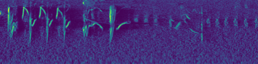
With the spectrogram image in hand, the next challenge is to apply transformations to the image to make it easier for the computer vision model to pick up on all the relevant pieces of the signal. In a raw spectrogram, the numerical values associated with a bird vocalization will often be very close to those associated with background noise. This is easiest to see by comparing a raw (mel-scaled) spectrogram to its original audio clip:
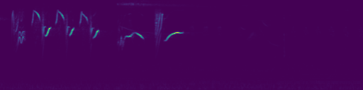
In this clip, some of the louder parts of the Lesser Goldfinch‘s song appear on the left hand side of the spectrogram. But there are some important sounds in the clip that are not visible in the raw spectrogram. For instance, there is an Allen’s Hummingbird buzzing in the middle of the clip, and a second Lesser Goldfinch singing in the second half of the clip. If you only had the raw spectrogram to go off of, you would not realize that these birds were present in the recording.
One solution is to nonlinearly rescale the values of the spectrogram to clearly separate the signal from the noise. A more sophisticated approach is to try to isolate the underlying background noise and remove it from the spectrogram using a per-channel energy normalization (PCEN) described below.
Different approaches to processing a spectrogram
Prior to additional processing, we normalized each spectrogram to take values between
Decibel: Replaces spectrogram values by their logarithm.
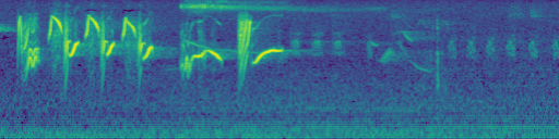
Exponential (Following Schlüter 2018): Replaces spectrogram values by a power.
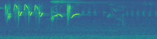
Per-Channel Energy Normalization (PCEN) (Following Wang et al. 2016): Combines a nonlinear scaling of spectrogram values (as in decibel and exponential frontends), with adaptive gain control. The adaptive gain control tries to predict the level of stationary background noise in each mel band, and then amplify the signal when it is greater than the background noise level. The mathematical details are described in this nice exposition. In PCEN there are five learnable parameters. They can be learned for the entire spectrogram, or a set of five parameters can be learned for each mel band individually.
A standard library implementation of PCEN introduces artifacts, as can be seen here:
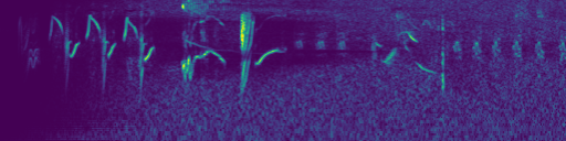
These artifacts come from a choice of initialization for the adaptive gain control. By looping the spectrogram in the time domain before applying PCEN, we were able to avoid these artifacts.
In some cases, frontends which combine PCEN with additional learnable parameters can outperform the ones we outlined above (see for instance, the LEAF frontend). We did not explore these approaches, for a couple of reasons. First, the modest performance gains reported did not seem to justify the engineering effort necessary for implementation. Second, we did not see dramatic improvement with PCEN alone, and we were skeptical that the additional learnable parameters would improve things. Some of these additional parameters control filter placement in the frequency domain, but we expect that the same benefit can be achieved by simply using a larger number of mel filters (for instance, 128 rather than 96).
Combinations thereof: An off-the-shelf computer vision model is designed to process images with three color channels (for the red, green, and blue components of each pixel). Since spectrograms have only one color channel, we had the option to either duplicate this channel three times, or to choose different processing settings for each channel individually. By using this second approach, we had the option of mixing and matching the different frontends described above to benefit from the strengths of multiple frontends.
Experiments
To compare the different spectrogram preprocessing frontends described above, we trained and tested a different model using each type of preprocessing. We describe the experimental setup in the previous post using our “best practices” spectrogram creation parameters. Models were trained on a 52 species dataset.
To illuminate the extent to which the performance of each of these models depends on the data we used, we evaluated each of these models on a second dataset, called SWAMP: Sapsucker Woods Acoustic Monitoring Project. The SWAMP test dataset is disjoint from the Merlin Sound ID test and train datasets, and consists of audio taken from autonomous field recorders from Sapsucker Woods in Ithaca, NY. Part of the motivation to use this second dataset came from the fact that the SWAMP recordings are characterized by a low ratio of signal to background noise. PCEN has been reported to drastically improve model performance in this type of acoustic context.
Here is an example recording (of an Eastern Towhee) from this dataset:
Audio PlayerWe choose a subset of three second clips from SWAMP so that each clip contained only birds contained in the 52 species training dataset.
The following compares performance on SWAMP, measured by mean average precision (MAP), to performance on our standard Merlin test dataset.
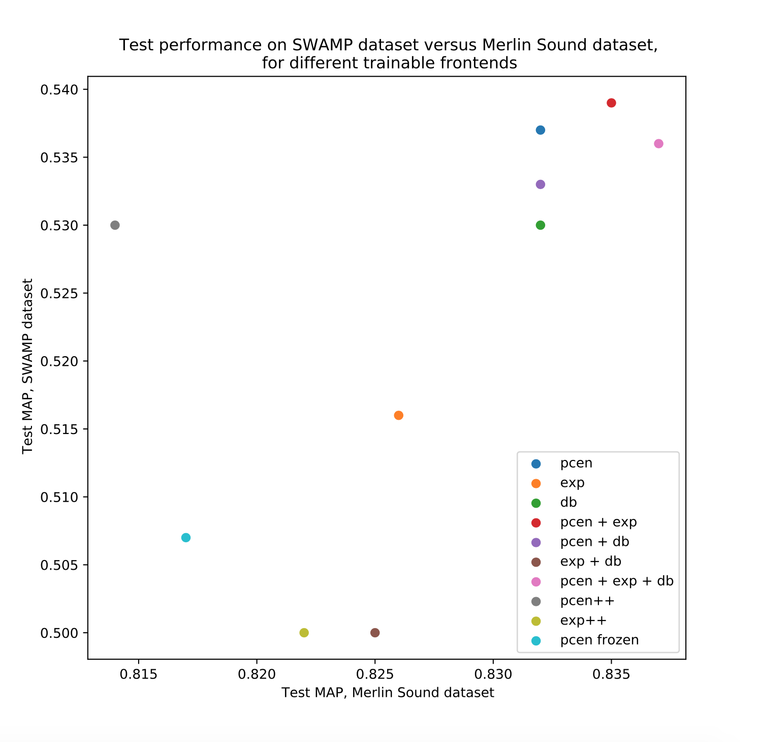
Between the top five models, there was little difference (less than one percent MAP) in test performance. This trend was present across both datasets we used for evaluation. In particular, the gains in performance achieved by PCEN and its variants were modest, as compared to decibel scaling. Each model performed much better (about 30 percent MAP) on the Merlin Sound ID dataset, as compared to the SWAMP dataset. This difference can be attributed to a higher sound quality in the Merlin Sound ID dataset, as well as label noise in the SWAMP dataset due to a less rigorous annotation protocol.
We did not, in all cases, estimate the variance in MAP that results from random initialization of parameters in training, dataset shuffling, and random spectrogram augmentations. However, based on a limited experiment (
A disadvantage of using a trainable PCEN frontend is that the mathematical operations used in PCEN include large matrix multiplications, which are computationally expensive, and element-wise divisions, which require a higher degree of numerical precision (32 bit rather than 16) than we typically used for model training. The result is that models using a trainable PCEN frontend took longer to train than models using decibel or exponential frontends. In some cases, training times increased by close to 50 percent. While this number could likely be decreased by improving our implementation, our skepticism about the magnitude of performance improvements promised by PCEN led us to pause this investigation for the time being.
Conclusions
Custom layers for spectrogram processing have received a lot of attention in the audio machine learning community. Approaches range from the ultra-classic (decibel scaling) to the ultra-fancy (frontends like LEAF). We tried several approaches which have been documented in the literature, and in the case of PCEN introduced some improvements to the library implementation. At the end of the day, we found that decibel scaling provides a strong baseline. This happens to be the same preprocessing that expert curators at the Macaulay Library use to visualize spectrograms, so it doesn’t come as a surprise that it works well for a CNN. Alternatives like PCEN may result in slight gains, but at the expense of longer training times. We found that model performance was more strongly governed by choices of architecture, loss function, and data augmentations.