

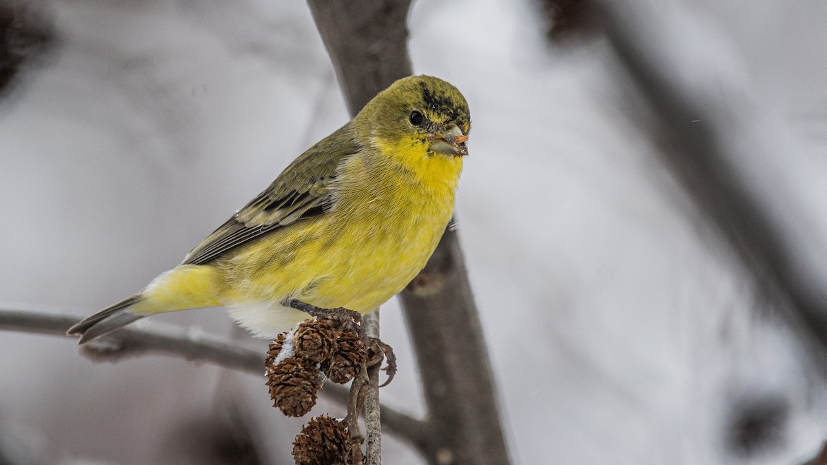
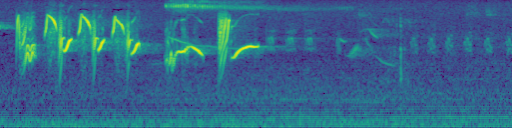
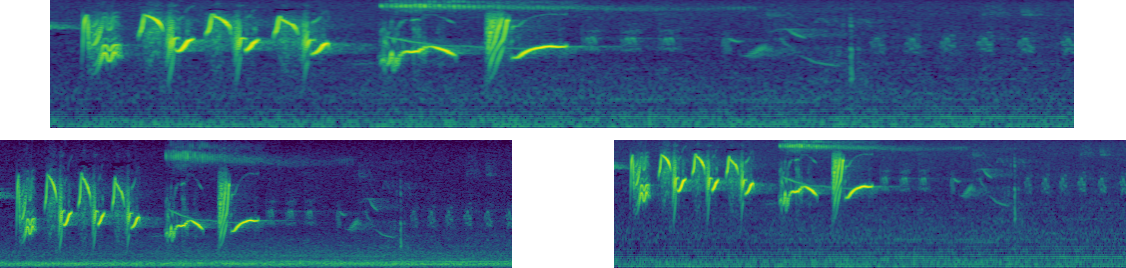
In our first post, we described the idea of using a computer vision model to identify bird vocalizations. But how does a computer vision model “listen” to a sound? For Sound ID, we use the short-time Fourier transform (STFT) to convert the raw waveform (which tracks air pressure as a function of time) into an image called a spectrogram. A spectrogram tracks the sound frequencies (vertical axis) which appear in the waveform, as a function of time (horizontal axis). Brighter colors correspond to louder sounds.
Once the audio has been converted into a spectrogram it can be fed into a standard computer vision model, which learns how to identify bird vocalizations based on their visual signature in the spectrogram. In this series of posts, we’ll look at what matters—and what doesn’t—when creating a spectrogram.
But why spectrograms?
Before jumping into the details of how we created and treated our spectrograms, we’ll mention a couple different approaches. The first of these alternatives is to work with the waveform directly. In this framework, the waveform, which is a series of air pressure samples, is fed directly into the computer’s classification model. This model could be a one-dimensional convolutional network, or could use some other architecture like a Transformer. The main disadvantage of using the waveform directly is that the relevant parts of the waveform, the parts that correspond to sounds we hear, are manifested as patterns that appear across hundreds or thousands of pressure samples. Because they are not localized in the waveform, they are hard to find. In principle, a model could learn a set of filters which pick up on certain frequencies, but in practice this will be hard for the model to do. An example of this approach, together with visualizations of the learned filters, can be found in this 2015 article by Palaz et al. By giving the model a spectrogram, we effectively shortcut the task of learning different filters to apply to the raw waveform.
Rather than working with waveforms directly, we have the option of representing our sound as an image either as a spectrogram or some other image representation. This approach has several advantages. First, image representations are indispensable tools for bird sound ID experts who are trying to identify species in a recording. For example, the Peterson Field Guide to Bird Sounds uses spectrograms as its main tool for describing bird vocalizations. By way of analogy, image representations should be useful for computers trying to perform the same task. Second, by using image representations, we have the option of using well-understood computer vision model architectures (e.g., ResNet), initialized with pre-trained weights from ImageNet or iNaturalist. The approach of using image representations of sound is standard in the machine listening research community (see for instance recent submissions to DCASE challenges).
There are alternative procedures to represent a waveform as an image other than the STFT. These procedures could be learned by the computer (as in LEAF, which we’ll discuss in the next post), or could be fixed (as in the wavelet scattering transform). With this kind of representation in hand, one could train a computer vision model to recognize the bird vocalizations that appear, just as we did with spectrograms. These other methods contain some beautiful ideas, and would be worth investigating further.
Spectrogram creation experiments
There are a number of choices one can make when constructing a spectrogram. Among them are the following:
• Clip length: How many seconds of audio should a spectrogram represent?
• STFT window length: Represents a tradeoff between a spectrogram’s level of resolution in the time domain (short window length) and resolution in the frequency domain (long window length).
• STFT hop size: A shorter hop size leads to higher resolution in the time domain, but results in larger inputs to the model. In turn, larger inputs may slow down model training and inference.
• Mel scaling: In a frequency spectrogram, the vertical distance that represents an octave is not constant. As a result, it may be difficult for convolutional filters to learn to recognize harmonies, overtones, and repeated harmonic patterns. Mel scaling rescales the frequency axis, so that fixed differences in musical pitch (e.g. an octave or a fifth) correspond to fixed vertical distances. One possible downside to using mel scaling is that high frequency sounds will become compressed at the top of the spectrogram, and therefore might be harder to distinguish.
• Image rescaling: Choices of the parameters above affect the spatial dimensions of the resulting spectrogram. To make meaningful comparisons, we chose a set of image dimensions to rescale our spectrograms to.
We compared the following configurations of parameters. All waveforms were taken at a rate of 22050 samples per second.
• Clip length: Based on preliminary experiments, we chose to use 3 second audio clips. We found that shorter clips often eliminated important context from the soundscape, while models using longer clips were more expensive to train.
• STFT window length: 256 or 512 samples
• STFT hop size: 64 or 128 samples
• Mel scaling: On or off
• Image rescaling: rescale to [128, 512] or [96, 512] (for hop size 128), or [128, 1024] (for hop size 64)
We performed a grid search across these parameters, using spectrograms with decibel scaling. We trained a ResNet-50, initialized with weights from ImageNet, for 90 epochs. The model was trained to perform multi-label classification, with a binary cross-entropy loss function. We used an SGD optimizer, with initial learning rate 0.1 and piecewise-constant learning rate decay. A variety of spectrogram augmentations were applied, which will be discussed in a future post. The following relates mean average precision (MAP) across 458 bird species, versus training time:
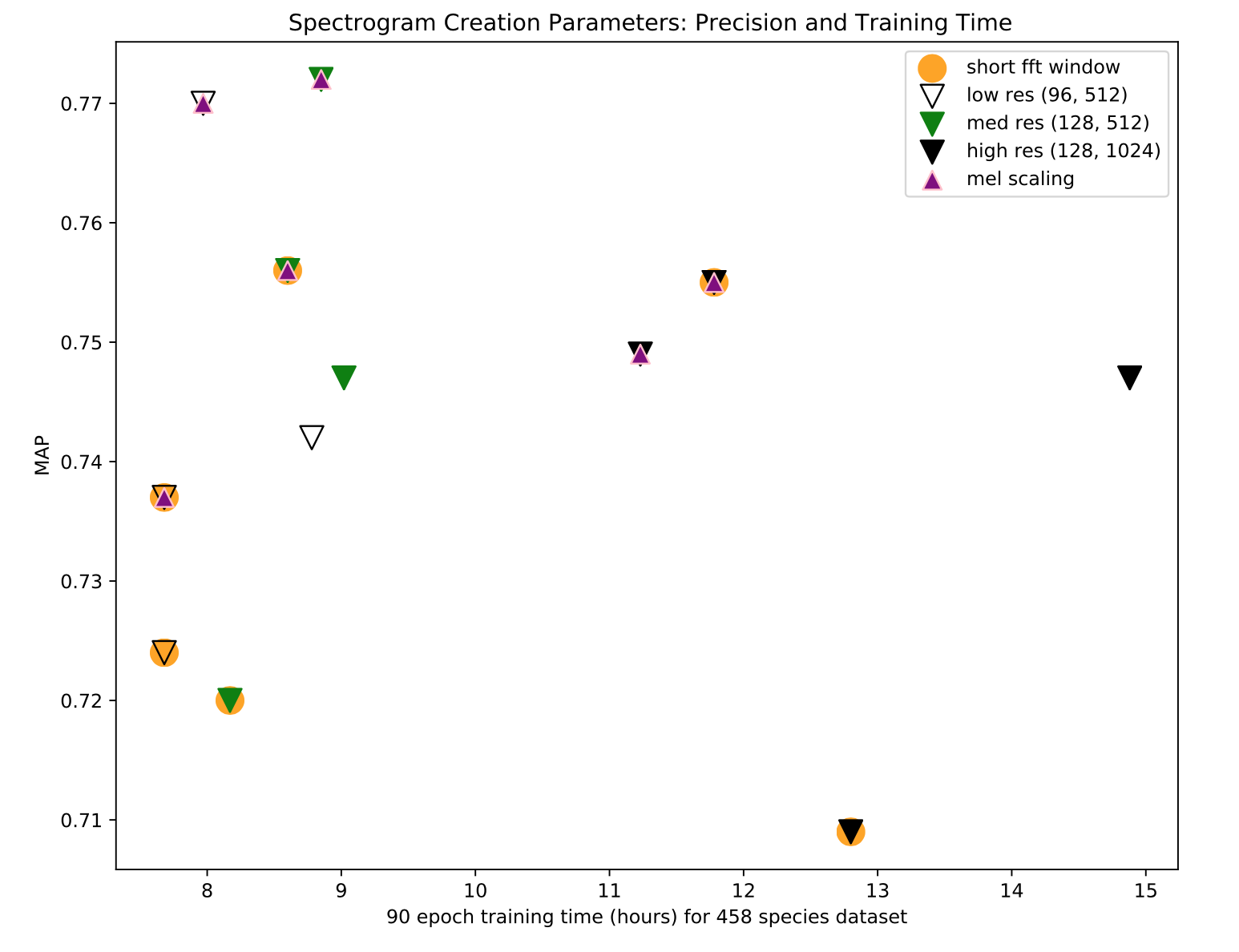
We identify three main takeaways: First, mel scaling uniformly does better than frequency scaling. Second, high resolution spectrograms lead to longer training times, as well as lower model performance. The decrease in performance is surprising, but we expect that it is related to a mismatch between the size of the convolutional filters in the ResNet, and the size of a semantically meaningful piece of the spectrogram. Third, the longer STFT window length performed uniformly better than the shorter window length we tested.
A wider sweep of these hyperparameters is clearly possible. We did not do an exhaustive sweep, and we adopted these as our best practices in experiments that followed.
• Window length: 512 samples
• STFT hop size: 128 samples
• Mel scaling: On
• Image size: [128, 512]
There is no general consensus about how to best construct a spectrogram. Through experimentation, we found a set of parameters which achieves a good balance between spectrogram creation speed and model performance. In the next post, we’ll take a look at different transformations that can be applied to a spectrogram before passing it through a convolutional neural network.